Example uses of autorej and matrix solvers in general.

Using all your information.

For about a year I interacted with a very interesting engineer living in India. I will call him C.H. He was working with well logging mostly. This means that instruments are lowered down an oil well which is being drilled, for the purpose of detecting properties of the surrounding earth. The instrument package emits various probing signals, and the surrounding earth responds in some fashion, depending on the nature of the probing signal: various wavelengths of radiation, and presumably certain radioactive materials, and I am not sure what else. Plus, I assume it measures easy to measure things such as temperature.

I am not sure exactly what the emitters and sensors were, because it didn’t matter to me. I was just trying to help him solve the difficult equation systems that resulted. One reason they were difficult is that this arrangement is in part a classic indirect sensing problem. Indirect sensing problems are often ill-conditioned due to the nature of trying reverse nature. In this case signals are emitted, which are basically a “diffusive” process. The signals spread out, and the observer can only measure certain effects of that diffusive process. Reversing nature’s stable processes such as heat flow is generally difficult, inaccurate, and unstable. Trying to calculate an earlier heat pattern in a material from an observed later, diffused heat patten is perhaps the most iconic example of such calculations, and inverse heat problems are perfect example problems of ill-conditioned systems. So they are used in testing algorithms like autorej uses.

Here is one of his matrix problems (a.k.a. linear algebra systems) that we worked on). The last column is the observations.

56.22	1070	1.95	4.78	0.015	303.44	28.8	8.4	8.57566
3.91	4.08	1.22	2.64	0.25	4.51	3.2	2.77	1.85502
0	0	0	0	0	4000	180	250	19.5
0	0	0	0.001	0	2000	8	35	4.75051
0	0.001	0	0.001	0	300	17	8	1.53051
0	0	0	0.001	0	0	0.1	6	0.065506

Here is the Picard Condition Vector for this problem (see the Tutorial for more on the PCV):

[0.00448 0.00669 0.04127 0.03892 0.34695 0.37723]

This is not a bad PCV at all, but it is a little odd as the first several values are very small, and the first, which is often the largest, is in fact the smallest. But I have seen this behavior in other contexts as well. Here is the solution (that would come any reasonable equation solver). I will show it graphically because the graphs convey the situation well here.

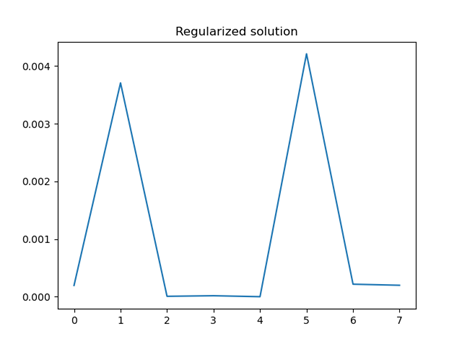
Kind of an interesting graph. The problem is that this is not at all what C.H. expected. The scale of the vertical axis is also too small. Discussing this, I realized that it was known that the solution values should add to 1. Autorej’s solve_constrained() accepts one constraint equation that is to be obeyed exactly: not as a normal least squares equation. To ask the sum to be 1.0 we set all the coefficients to 1, creating a sum, and set the right hand side value to 1, which is the sum we want.

[ 1.0 1.0 1.0 1.0 1.0 1.0 1.0 1.0 ], with b=1.0

Here is the result:

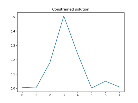
Wow! What a difference! Almost shockingly different… and much more reasonable and as expected. So be sure and ask yourself, if you are having difficulty getting a good solution, if you have included all the data you have.

I should mention to you that the algorithms in autorej could be much more general than provided here, but we have chosen to include only the most common features. For example, my C++ library allows any number of such “equality” constraints, and any number of inequality constraints, such as equations that ask a particular value to be no less than 10.0, for example, or for the sum to be not over 5, etc.